The Quantum Dimension
Introductions
Background
As many a great adventure, it all began with a few free credits. How it ended? Well you will just have to continue reading on.
A sign of my failing social life, one evening I was browsing the Azure Services looking to see what I could play with next and found the rather cool sounding Azure Quantum. Now, while Quantum is no longer in trend, and I believe that it’s currently in the pit of despair, Quantum would seem cool again very soon. Just like blockchain may one day soon. If that doesn’t make sense, check out Gartner’s Tech Hype Cycle.
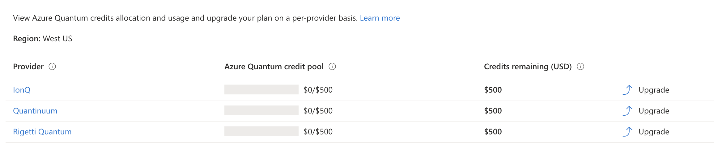
More importantly, and my wallet feeling fragile from Azure’s monthly billing offensive, they were giving away some free credits…I’m sold, let's mess around.
The Why?
From my very superficial understanding, Quantum computing is very good at those really tough calculations, while computers require linear amounts of compute to solve them, Quantum lives on an exponential domain. Very simply, Quantum is very good at optimisation.
Now I just needed to find something to optimise. In the utilities world, you might immediately think of a use case along the lines of optimising the scheduling of generation assets (and DERs) across multiple parameters (cost, emissions, fuel consumption, value etc.) across millions of units. If we are thinking on a bigger scale, even full power grid optimisation using plant, consume, transmission line data.
In the finance world, perhaps the optimisation of a portfolio comes to mind. Or maybe even energy trading (back to utilities).
I would love to test this use case out, unfortunately I don’t have that real life data collected, and aggregated, yet.
However, with the help of my friend, Copilot, I was able to whip up a dummy set of data in no time.
So what's Quantum good at?
From my very superficial understanding, Quantum computing is very good at those really tough calculations, while computers require linear amounts of compute to solve them, Quantum lives on an exponential domain. Very simply, Quantum is very good at optimisation.
Now I just needed to find something to optimise. In the utilities world, you might immediately think of a use case along the lines of optimising the scheduling of generation assets (and DERs) across multiple parameters (cost, emissions, fuel consumption, value etc.) across millions of units. If we are thinking on a bigger scale, even full power grid optimisation using plant, consume, transmission line data.
In the finance world, perhaps the optimisation of a portfolio comes to mind. Or maybe even energy trading (back to utilities).
I would love to test this use case out, unfortunately I don’t have that real life data collected, and aggregated, yet.
However, with the help of my friend, Copilot, I was able to whip up a dummy set of data in no time.
The Experimentation
Scenario #1
Baby steps, starting it simple
Scenario Details
We have a set of N power plants (sources), and M consumers. We have 3 Sources: ["A1", "A2", "A3"] We have 4 Consumers: ["B1", "B2", "B3", "B4"]
Desired outcome
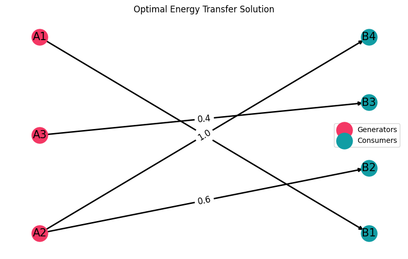
The goal is to supply power to all consumers, meeting the constraints of the power plants, and minimize the total cost of supplying power.
Discussion Points:
Step #1: The Mathematic Representation
Step #2: Articulating the problem
Step #3: Solving with Quantum (Simulation)
Step #4: Solving with Quantum (Real deal)
Quick admin - install the libraries
    from itertools import product
    import matplotlib.pyplot as plt
    import networkx as nx
    import numpy as np
    from qiskit import *
    from qiskit.visualization import plot_histogram
    from qiskit_algorithms import QAOA
    from qiskit_optimization.algorithms import MinimumEigenOptimizer
    from qiskit_algorithms.optimizers import COBYLA
    from qiskit_optimization import QuadraticProgram
    from qiskit_aer.primitives import Sampler
    from qiskit_aer import Aer
As you can see, we are using IBM's qiskit quantum library
Articulating the Problem
cost_matrix = np.array(
    [[0.5, 1.0, 1.0, 2.1], [1.0, 0.6, 1.4, 1.0], [1.0, 1.4, 0.4, 2.3]]
)
Sources = [“A1”, “A2”, “A3”]
Consumers = [“B1”, “B2”, “B3”, “B4”]
N = len(Sources)
M = len(Consumers)
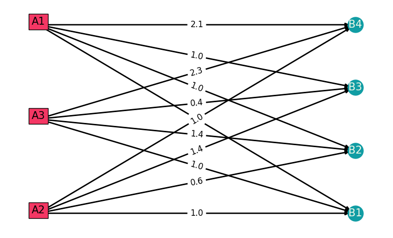
The cost_matrix defines the per-unit transmission costs from each power plant (source) to each consumer. Specifically, each row corresponds to a source (A1, A2, A3) and each column corresponds to a consumer (B1, B2, B3, B4). For example, the cost from source A1 to consumer B1 is 0.5, while the cost from source A1 to consumer B4 is 2.1.
Solving with Quantum (Simulation)
1. Define the Optimization Problem
problem = QuadraticProgram()
for i in range(N):
  for j in range(M):
    problem.binary_var(name=f"x_{i}_{j}")
problem = QuadraticProgram()
This creates an empty optimization problem where you'll later add variables, constraints, and an objective.
The loop over i (from 0 to N-1) and nested loop over j (from 0 to M-1) create a grid of decision variables.
For each combination of i and j, a binary variable is added to the problem.
The variable name is set to "x_{i}_{j}" (using an f-string for string interpolation), which helps identify its corresponding source (i) and consumer (j).
These variables typically represent decisions—in this case, whether to supply power from source A_i to consumer B_j—and can only take the values 0 or 1. This structure is useful in problems like assignment or network flow where a binary decision is needed at each pairing.
2. Build and Set the Objective
Build the objective as a dictionary mapping variable names to their cost coefficients
    objective_linear = {}
    for i in range(N):
      for j in range(M):
        objective_linear[f"x_{i}_{j}"] = cost_matrix[i, j]
    # Objective function: minimize the cost
    problem.minimize(linear=objective_linear)
objective_linear = {}This dictionary will store each decision variable (by name) paired with its cost coefficient.
      for i in range(N):
      for j in range(M):
        objective_linear[f"x_{i}_{j}"] = cost_matrix[i, j]
Two nested loops iterate over all combinations of i (for sources) and j (for consumers). For each pair, the code creates a key "x_{i}_{j}" (corresponding to the binary variable defined earlier) and assigns it the value from cost_matrix[i, j]. This maps each decision variable to its associated cost.
          objective_linear = {'x_0_0': 0.5,
        'x_0_1': 1.0,
        'x_0_2': 1.0,
        'x_0_3': 2.1,
        'x_1_0': 1.0,
        'x_1_1': 0.6,
        'x_1_2': 1.4,
        'x_1_3': 1.0,
        'x_2_0': 1.0,
        'x_2_1': 1.4,
        'x_2_2': 0.4,
        'x_2_3': 2.3}
problem.minimize(linear=objective_linear)This tells the optimizer that the goal is to minimize the total cost as represented by the sum of the costs times the decision variables. In other words, it adds up each variable's cost coefficient (multiplied by the value of that variable, which will be 0 or 1) to form the objective.
3.1 Consumer Supply Constraint
      # Constraint: Each consumer must be supplied by exactly one source
      for j in range(M):
        problem.linear_constraint(
          linear={f"x_{i}_{j}": 1 for i in range(N)},
          sense='==',
          rhs=1,
          name=f"cons_{j}" #name he constraint
        )
The loop iterates once for each consumer (indexed by j). For every consumer, a constraint will be added. The coefficient 1 for each variable indicates that every decision variable (whether a link from a source to consumer j) is equally weighted in the constraint.
For each consumer (each value of j), this code adds a constraint that collects all decision variables for that consumer (one for each source) and requires their sum to be exactly 1. This models the requirement that every consumer must be supplied by exactly one source.
3.2 Source Capacity Constraint
      # Constraint: Each source can supply a maximum of 2 units of power
      for i in range(N):
        problem.linear_constraint(
          linear={f"x_{i}_{j}": 1 for j in range(M)},
          sense='<=',
          rhs=2,
          name=f"source_{i}")
Where each consumer is assumed to consume 1 unit of power e.g. a source can only supply up to two consumers
4. Set Up the Quantum Algorithm
    # Set up the quantum algorithm with appropriate sampler and optimizer
    sampler = Sampler()
    sampler.options.backend = Aer.get_backend("qasm_simulator")
    optimizer_cobyla = COBYLA()
    qaoa = QAOA(sampler=sampler, optimizer=optimizer_cobyla, reps=1)
# Wrap QAOA in the MinimumEigenOptimizer
min_eigen_optimizer = MinimumEigenOptimizer(qaoa)
sampler = Sampler()
sampler.options.backend = Aer.get_backend(“qasm_simulator”)
The Sampler() object is used to sample outcomes from the quantum circuit. The backend is set to IBM’s Aer QASM simulator, which simulates quantum measurements on a quantum computer.
optimizer_cobyla = COBYLA()COBYLA() is a classical optimizer that is often used with quantum algorithms to adjust circuit parameters iteratively.
qaoa = QAOA(sampler=sampler, optimizer=optimizer_cobyla, reps=1)QAOA (Quantum Approximate Optimization Algorithm) is a hybrid quantum-classical algorithm designed to solve optimization problems. Basically magic It is configured with the quantum sampler and the classical optimizer. The parameter reps=1 sets the depth (number of repetitions) of the QAOA circuit; increasing this value can sometimes improve solution quality at the cost of longer execution time.
min_eigen_optimizer = MinimumEigenOptimizer(qaoa)The MinimumEigenOptimizer wraps the QAOA instance so that it can be used to solve optimization problems formulated as quadratic programs. Essentially, it leverages QAOA to find the minimum eigenvalue (solution) of the problem’s cost function, thereby determining the optimal (or near-optimal) assignment for the decision variables.
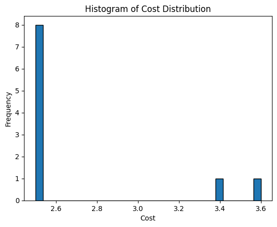
5. Execute Multiple Runs and Collect Results
# Perform multiple runs to collect a distribution of results
num_runs = 10  # Number of runs
results = []
for _ in range(num_runs):
  result = min_eigen_optimizer.solve(problem)
  best_cost = result.fval
  results.append(best_cost)
The loop iterates 10 times. In each iteration, the min_eigen_optimizer.solve(problem) call attempts to solve the optimization problem using the quantum algorithm (QAOA). The result.fval accesses the final cost (objective function value) of the solution. That cost is then appended to the results list.
Step #4: Solving with Quantum (Real deal)
Pending free time
Scenario #2
Trying something different and failing....
Scenario Details
The objective of this optimization model is to minimize the total cost of generation while meeting a specified total generation capacity (10,000 kW) . The algorithm needs to determine how much capacity to allocate to each of the 100 available generation assets, considering:
- Individual asset costs: ranging from 10–100 units
- Maximum capacity constraints: ranging from 50–500 kW per asset
- Total generation demand: 10,000 kW
This is achieved using the Markowitz Portfolio Optimization approach , which balances cost minimization with capacity constraints to find the most economically efficient allocation of generation resources.
Discussion Points:
Step #1: The Mathematic Representation
Step #2: Articulating the problem
Step #3: Solving Classically
Step #4: Solving with Quantum (Simulation)
Step #5: Solving with Quantum (Real deal)
Step #2: Classical Optimisation
Libraries & Data Generation
    import numpy as np
    import pandas as pd
    import matplotlib.pyplot as plt
    from scipy.optimize import minimize
    # Generate random data for 100 generation assets
    np.random.seed(42)
    num_assets = 100
    costs = np.random.uniform(10, 100, num_assets)  # Random costs between 10 and 100
    max_kw = np.random.uniform(50, 500, num_assets)  # Random max kw between 50 and 500
    # Create a DataFrame to hold the data
    assets_df = pd.DataFrame({
        'Cost': costs,
        'Max_kW': max_kw
    })
Defining the Optimization Setup
    # Define the expected returns (negative cost for minimization)
    expected_returns = -assets_df['Cost'].values
    # Define the covariance matrix (assuming independent assets for simplicity)
    cov_matrix = np.diag(np.ones(num_assets))
    # Define the constraints: sum of allocations should be equal to total generation capacity
    total_generation_capacity = 10000  # Example total generation capacity in kW
    constraints = ({'type': 'eq', 'fun': lambda x: np.sum(x) - total_generation_capacity})
    # Define the bounds: allocation should be between 0 and max_kw for each asset
    bounds = [(0, max_kw[i]) for i in range(num_assets)]
The Optimisation Process
# Define the objective function: minimize the negative expected returns (maximize returns)
def objective_function(weights):
return -np.dot(weights, expected_returns)
# Perform the optimization using Markowitz Portfolio Optimization
result = minimize(objective_function, np.ones(num_assets) * total_generation_capacity / num_assets,
method='SLSQP', bounds=bounds, constraints=constraints)
# Get the optimal allocation
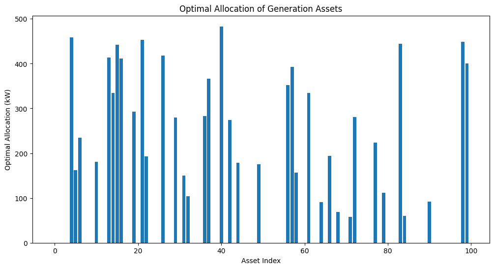
optimal_allocation = result.x
The Outcome
Total Cost: 234198.7958920941
Total Generation: 10000.000000022186
Step #4: Solving with Quantum (Simulation)
e.g. Going Quantum
Setting up the libraries
      from dimod import SimulatedAnnealingSampler, BinaryQuadraticModel
      import numpy as np
      import pandas as pd
Setting up the problem
      scale_cost = 1e7
      # Define the QUBO matrix for the problem
      Q = {}
      for i in range(num_assets):
          for j in range(num_assets):
              if i == j:
                  # Cost factor for each asset (objective term)
                  Q[(i, j)] = scale_cost * costs[i]
              else:
                  # Assuming no correlations between assets
                  Q[(i, j)] = 0
  # Add constraints to enforce the total generation capacity
  penalty = 1e8 # A large penalty value for constraint violation
  for i in range(num_assets):
      Q[(i, i)] += -penalty * max_kw[i]  # Penalizing allocations exceeding max_kW
  for i in range(num_assets):
      for j in range(i, num_assets):
          Q[(i, j)] += penalty * (max_kw[i] * max_kw[j]) / total_generation_capacity
Solving the problem using Annealing
# Solve the QUBO using the simulated annealing sampler
sampler = SimulatedAnnealingSampler()
response = sampler.sample_qubo(Q, num_reads=5)
# Extract the optimal solution (binary)
optimal_solution = response.first.sample
# Convert binary solution to actual allocations (kW)
optimal_allocation_quantum = [optimal_solution[i] * max_kw[i] for i in range(num_assets)]
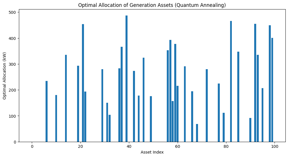
assets_df['Optimal_Allocation_kW_Quantum'] = optimal_allocation_quantum
The Outcome
A bit crap - I suspect it's due to my scaling. Spent an hour or so messing around, but then gave up. Maybe increasing the runs on the Quantum Computing will help. Perhaps once I truly know what I'm doing I'll come back to it.
Quantum Approach: Total Cost = 305441.67304096126, Total Generation = 9729.458504587521
Step #5: Solving with Quantum (Real deal)
Pending some free time